Introduction
My personal favorite neural network. It solved the vanishing gradient problem by avoiding it all together and is incredibly useful for time-dependent data. The training set is the stock prices of Google from 2012-2016 and the goal is to predict the actual stock prices of 2017, which will be the test set.
Code
Like other deep learning models I have seen, the training process was completed differently since the dependent variable won’t just be based on the independent data in its row in the csv file. The process can be seen below.
X_train = []
y_train = []
for i in range(60, 1258): #Collecting the financial data for the amount of days in the training set
    X_train.append(train_scaled[i-60:i, 0])
    y_train.append(train_scaled[i,0])
X_train, y_train = np.array(X_train), np.array(y_train)
After collecting the data, it was time to build the LSTM model. It was surprisingly similar to other models I have seen, such as ANN or CNN, however dropout was utilized to prevent overfitting. This could be especially dangerous since there was a relatively small data set to train the model.
#Building RNN
from keras.models import Sequential
from keras.layers import Dense
from keras.layers import LSTM
from keras.layers import Dropout

regressor = Sequential()
#Layer 1
regressor.add(LSTM(units = 65, return_sequences = True, input_shape =(X_train.shape[1], 1)))
#Dropout regularization
regressor.add(Dropout(0.2))

#Layer 2
regressor.add(LSTM(units = 65, return_sequences = True))
regressor.add(Dropout(0.2))

#Layer 3
regressor.add(LSTM(units = 65, return_sequences = True))
regressor.add(Dropout(0.2))

#Layer 4
regressor.add(LSTM(units = 65, return_sequences = False))
regressor.add(Dropout(0.2))

#Adding output layer
regressor.add(Dense(units = 1))

#Compile
regressor.compile(optimizer = 'adam', loss = 'mean_squared_error')
Results
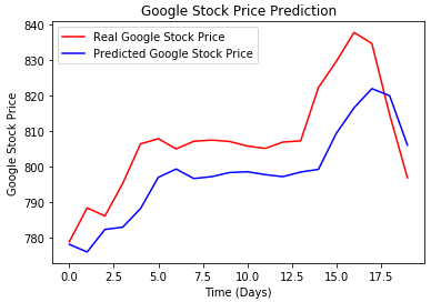
It was finally time to test the validity of not only the model, but the optimizer used in compiling as well. I gathered the test data the same way I gathered the training data using for loops, then plot them.
#Predicted prices of 2017
data_total = pd.concat((data_train['Open'], data_test['Open']), axis = 0) #Bringing entire data set together so proper prediction making can happen
inputs = data_total[len(data_total)-len(data_test)-60:].values #Predictions are based off the 60 previous days so that is what is being implemented here
inputs = inputs.reshape(-1,1) #Reshape into numpy friendly array
inputs = sc.transform(inputs) #Allows for scaling of the inputs the same way the training set was scaled without chaning the actual data
X_test = [] #Same as the first block of code on the page however goes from 60-80 since there are only 20 financial days to look at in the test data
for i in range(60, 80):
    X_test.append(inputs[i-60:i, 0])
X_test = np.array(X_test) #Changes into numpy array
X_test = np.reshape(X_test, (X_test.shape[0], X_test.shape[1], 1))
predicted_stock_price = regressor.predict(X_test) #Prediction time however it is a regressor since it is continuous data we are finding
predicted_stock_price = sc.inverse_transform(predicted_stock_price) #Undo the scaling

#Visualization
plt.plot(real_prices, color = 'red', label = 'Real Google Stock Price')
plt.plot(predicted_stock_price, color = 'blue', label = 'Predicted Google Stock Price')
plt.title('Google Stock Price Prediction')
plt.xlabel('Time (Days)')
plt.ylabel('Google Stock Price')
plt.legend()
plt.show()
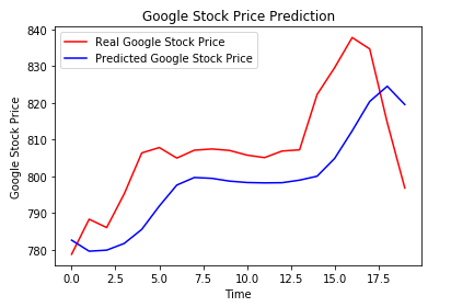
It’s a close race, so looking at the mean squared error would help give a better idea of the results.


Looking at the rmse really showed how close the models were when it came to training. The difference may be scaled along with the size of the data, however I found both to be acceptable for the set.