Introduction

Restricted Boltzmann Machines have been the most difficult type of neural network that I have encountered mainly because of how unique it is. Up until this point I have seen visible layer, hidden layer, then an output layer, so the idea of having a return without an output layer was difficult to grasp initially. From my understanding, one of the uses for RBM’s is for suggestions. Without trying to reinvent the wheel too much, I decided to use RBM’s to predict whether or not a user would like a movie based off their ratings of others. I downloaded my dataset from Grouplens, and began my work.

Code

The data preprocessing phase was relatively straight-forward with cleaning separating the data. The only real difference is that I used Pytorch for the first time. This required me to convert the training and test set into arrays readable by this library.

#Convert data into array that is usable by BM
def convert(data):
    list_of_lists = []
    for id_users in range(1, num_users + 1):
        id_movies = data[:,1][data[:,0] == id_users]
        id_ratings = data[:,2][data[:,0] == id_users]
        ratings = np.zeros(num_movies)
        ratings[id_movies - 1] = id_ratings
        list_of_lists.append(list(ratings))
    return list_of_lists
ts = convert(ts)
tst = convert(tst)

#Convert data into torch tensor
ts = torch.FloatTensor(ts)
tst = torch.FloatTensor(tst)

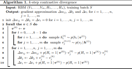
After converting the dependent variable, the scores given by the users, into binary I was ready to construct my neural network. This paper was my guide in creating and understanding how this model works. One of the more digestible methods in the paper is calculating the log-likelihood gradient using contrastive divergence. From the paper, I used the following algorithms to create a class that calculates my weights, biases, and takes samples of the hidden layers.

#Creating Neural Network
class RBM():
    def __init__(self, nv, nh): #self referal for objects in class, number of hidden and visible nodes. Nv= movies and nh = # of features
        self.W = torch.randn(nh, nv) #initializes weights tensor of size nh and nv
        self.a = torch.randn(1, nh) #initializes weights of each bias in reference to the batch (1) and the hidden node
        self.b = torch.randn(1, nv)
    def sample_h(self, x): #Samples activation of hidden nodes. X is the visible neurons
        wx = torch.mm(x, self.W.t()) #Nodes multiplied by weights
        activation = wx + self.a.expand_as(wx) #Applying bias to each line of minibatch
        p_h_given_v = torch.sigmoid(activation)#Probability that activation function is activated where v is the score and h is the genre
        return p_h_given_v, torch.bernoulli(p_h_given_v) #Returns probabilities and samples of hidden neurons
    def sample_v(self, y):#Samples activation of hidden nodes. X is the visible neurons
        wy = torch.mm(y, self.W) #No transpose because you are taking pv|h
        activation = wy + self.b.expand_as(wy) #Applying bias to each line of minibatch
        p_v_given_h = torch.sigmoid(activation)#Probability that activation function is activated where v is the score and h is the genre
        return p_v_given_h, torch.bernoulli(p_v_given_h) #Returns probabilities and samples of hidden neurons
    def train(self, v0, vk, ph0, phk):
        self.W += (torch.mm(v0.t(),ph0) - torch.mm(vk.t(),phk)).t()
        self.b += torch.sum((v0 - vk), 0)
        self.a += torch.sum((ph0 - phk), 0)

Results

The training process was the most unique out of all the other experiences, since it is based off sampling batches. 2 sets of visible nodes are created with one that is the control and another that is updated based on predictions from Gibbs sampling. The k-step loop updates the hidden layer based on the visible layer, then updates the visible nodes all while ignoring the users that skipped some of the ratings. The model was then trained, and the difference of the values of the control and updated visible nodes were taken to find a loss value. The training model was based off equations 8, 9, and 10 from the algorithm given above.

nb_epoch = 20
for epoch in range(1, nb_epoch + 1):
    train_loss = 0 #error
    s = 0. #counter
    for id_users in range(0, num_users - batch_size, batch_size): #Samples the user values in batches of 100
        vk = ts[id_users:id_users+batch_size] #Gibbs chain vector updated by every random walk (k steps)
        v0 = ts[id_users:id_users+batch_size] #Vector that will not be updated to compare and find error
        ph0,_ = rbm.sample_h(v0) #Probability the value of the hidden node equals 1 given real ratings
        for k in range(10): #K-steps of contrastive divergence
            _,hk = rbm.sample_h(vk) #samples the kth hidden node given the values of the visible nodes (actual ratings)
            _,vk = rbm.sample_v(hk) #updated the visible node after a round of Gibbs sampling of hidden nodes
            vk[v0<0] = v0[v0<0] #Ignores the nodes with a -1 rating (User did not give rating on moving)
        phk,_ = rbm.sample_h(vk) #Updates the probability value
        rbm.train(v0, vk, ph0, phk)
        train_loss += torch.mean(torch.abs(v0[v0>=0] - vk[v0>=0])) #update to the loss value
        s += 1. #update the counter
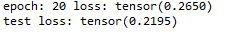
    print('epoch: '+str(epoch)+' loss: '+str(train_loss/s))

In both training and testing, I had a relatively low loss value, which I would chalk up as a success.

Restricted Boltzmann Machine

Najee Smith

Introduction

Code

Results