Introduction
Kernel SVM was one of the first classifiers that caught my attention mainly because it was both great at avoiding overfitting and useful for more practical non-linear data. Around the same time I learned about this, I had also found out about dimensionality reduction techniques, and figured it would be beneficial in not only practice both, but to compare and contrast them as well. The technique I chose is Kernel Principle Component Analysis. For obvious reasons both will use the same data set that lists customers’ information and whether or not they purchased an SUV because of its advertisement.
Code
Kernel SVM
The data was broken into 2 features, age and salary. Scaling was applied due to the large variation within the salary feature. The preprocessing step was nothing too strenuous since my goal of this project was to learn about what make these methods unique. The following I left the arguments relatively default with this same rationale.
from sklearn.svm import SVC
classifier = SVC(kernel = 'rbf', random_state = 0)
classifier.fit(X_train, y_train)
Dimensionality Reduction
I used logistric regression in tangent along reduction since the point of changing the dimensionality of the data was to make it linearly separable.
# Applying Kernel PCA
from sklearn.decomposition import KernelPCA #linearize data
kpca = KernelPCA(n_components = 2, kernel = 'rbf')
X_train = kpca.fit_transform(X_train)
X_test = kpca.transform(X_test)

# Fitting Logistic Regression to the Training set
from sklearn.linear_model import LogisticRegression
classifier = LogisticRegression(random_state = 0)
classifier.fit(X_train, y_train)
Results
Here, I plot the results with matplotlib for a visual analysis, and used a confusion matrix for a numerical one.
from matplotlib.colors import ListedColormap
X_set, y_set = X_test, y_test
X1, X2 = np.meshgrid(np.arange(start = X_set[:, 0].min() - 1, stop = X_set[:, 0].max() + 1, step = 0.01), #Creates limits for graph
                     np.arange(start = X_set[:, 1].min() - 1, stop = X_set[:, 1].max() + 1, step = 0.01))
plt.contourf(X1, X2, classifier.predict(np.array([X1.ravel(), X2.ravel()]).T).reshape(X1.shape), #Creates predicted binary regions
             alpha = 0.75, cmap = ListedColormap(('red', 'green')))
plt.xlim(X1.min(), X1.max())
plt.ylim(X2.min(), X2.max())
for i, j in enumerate(np.unique(y_set)): #Plots the data points and hopefully puts them in the correct regions
    plt.scatter(X_set[y_set == j, 0], X_set[y_set == j, 1],
                c = ListedColormap(('red', 'green'))(i), label = j)
plt.title('Logistic Regression (Test set)')
plt.xlabel('Age')
plt.ylabel('Estimated Salary')
plt.legend()
plt.show()

from sklearn.metrics import confusion_matrix
cm = confusion_matrix(y_test, y_pred)
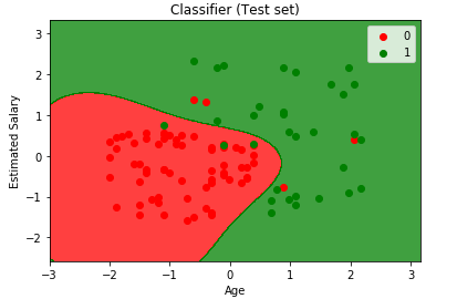
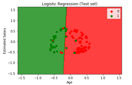
Both models were rather convincing to be useful since both graphs organize the customers in the correct predicted regions, however I’d rather not strain my eyes trying to count all the incorrect points. This is where simple math and a confusion matrix came into play.
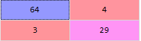
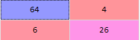
By adding the bottom left and upper right cells on each, it can be seen that Kernel SVM had only 7 incorrect predictions, while the Kernel PCA method had 10. I am completely aware this is only one project with a single data set, however I felt it was still a worthwhile comparison. Larger data sets would probably have an different results since Kernel SVM accuracy have an inverse relationship with data size.