K-Means Clustering

Introduction

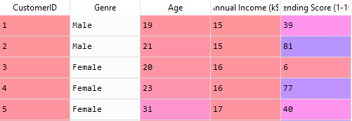
Another “sort-of” classifier that I had worked on. The significance of this was that it is a good thing to know especially if there is no direct dependent variable, but it also allowed for me to perform parameter tuning without using techniques such as grid search. The clustering process will be done on a data set from Kaggle that separates customers by age, salary, and spending score as shown below. The goal is to clusters of buyers of varying probability of purchasing an item.

Code

The task of determining the optimal number of clusters turned out to be less daunting than I imagined. In short, this was done by running a for loop to find the variance for having 1-10 clusters. The optimal number of cluster was chosen by both having a low wCSS (variance) and rate of change closest to 0, since any number of clusters after that would split the data too much, and the grouping would lose significance.

from sklearn.cluster import KMeans
wCSS = []
for i in range(1,11):
    kmeans = KMeans(n_clusters = i, init = 'k-means++', max_iter = 300, n_init = 10)
    kmeans.fit(X)
    wCSS.append(kmeans.inertia_) #Collects all of the within cluster sum of squares
plt.plot(range(1,11), wCSS)
plt.title('Elbow Method')
plt.xlabel('Clusters')
plt.ylabel('wCSS')
plt.show()

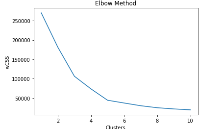
Here, 5 clusters seems to be optimal based on the criteria mentioned earlier. I chose the values for the parameters for the following reasons:

• init - K-means++ is a cleaner way of initializing centroid values

• max_iter - Left default to allow algorithm to optimize centroids along with n_init

• n_init - Also left as default since any value lower than this would not find optimal centroid seeds, while any value higher would be inefficient since the optimal seed would be captured in earlier iterations

Results

Now that an optimal number of clusters was found, it will be fit to the data set, then plotted.

kmeans = KMeans(n_clusters = 5, init = 'k-means++', max_iter = 300, n_init = 10)
y_kmeans=kmeans.fit_predict(X)

#Visualizing clusters
plt.scatter(X[y_kmeans == 0, 0], X[y_kmeans == 0,1], s=100, c='blue', label = 'C1')
plt.scatter(X[y_kmeans == 1, 0], X[y_kmeans == 1,1], s=100, c='red', label = 'C2')
plt.scatter(X[y_kmeans == 2, 0], X[y_kmeans == 2,1], s=100, c='green', label = 'C3')
plt.scatter(X[y_kmeans == 3, 0], X[y_kmeans == 3,1], s=100, c='yellow', label = 'C4')
plt.scatter(X[y_kmeans == 4, 0], X[y_kmeans == 4,1], s=100, c='purple', label = 'C5')
plt.scatter(kmeans.cluster_centers_[:,0],kmeans.cluster_centers_[:,1], s=300, c='black', label = 'Centroid')
plt.title('Clusters of Clients')
plt.xlabel('Income')
plt.ylabel('Score')
plt.legend()
plt.show()

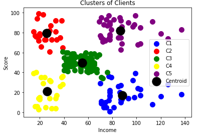
From this colorful graph, we have the 5 groups of customers gathered. From here, it could be up to the mall to either email sales advertisements to the people who lie in clusters 1 or 5 more than customers from 1 or 4 in order to increase profit.